SIGGRAPH 2026 · ACM Transactions on Graphics
Soft Anisotropic Diagrams
for Differentiable Image Representation
Laki Iinbor1 · Zhiyang Dou2,∗ · Wojciech Matusik2,∗
1Independent Researcher 2MIT ∗Joint last author
We represent an image as a set of adaptive anisotropic sites. Every pixel is a temperature-controlled softmax over its eight nearest sites under one score, ‖x − p‖G − r. The per-site temperature is the whole trick: it turns a blurry blend into crisp, content-aligned edges, so one small local computation renders and fits both.
Try it
Up to 64 sites, eight candidates per pixel, one score. Drag a site and the render follows. Press Fit to target and the same parameters are optimised in your browser with Adam, exactly as in the paper — positions, colours, radii, temperatures and anisotropy are all learnable. The fit runs on a 128×128 copy of the target.
Soft blend over the top-8 sites per pixel.
Target
View
Try this: drop τ low and the render turns into an averaged blur, even where the target has a hard edge. Raise it and the blend collapses onto the cell view — that convergence is what the temperature buys, and it is what lets one representation hold a sharp edge and a smooth gradient at once. The render above the sliders is the continuous model, redrawn from the site parameters on every frame, so the fit and what you drag are the same thing. Fitting 64 sites on the Text target is the most convincing setting; with 40 sites on the disc, levelling τ and radius first is worth the detour.
Fitting
Four runs, left to right: the reconstruction, hard cell ownership, and the learned temperature field. Sites migrate toward edges and texture, and τ resolves into warm seams along structure and cool fields across smooth gradients.
Reconstruction · cell ownership · log τ over site position. Played at 1.5×.
Results
At matched bitrate SAD is ahead of Image-GS and Instant-NGP on every dataset we evaluated, and the margin comes from the representation rather than from extra budget: the same site count buys sharper edges because temperature is decoupled from reach.
Grey dashed: baselines. Coloured dashed: further reference points. All metrics in linear colour space.
Kodak · 50k sites
| Method | PSNR | Time |
|---|---|---|
| Image-GS | 36.90 | 28 s |
| Instant-NGP | 37.72 | 8.2 s |
| Fast 2DGS | 43.13 | 10 s |
| SAD | 46.00 | 2.2 s |
+2.87 dB over Fast 2DGS at 4.5× less encoding time; 13× faster than Image-GS at the same quality protocol.
Training speed
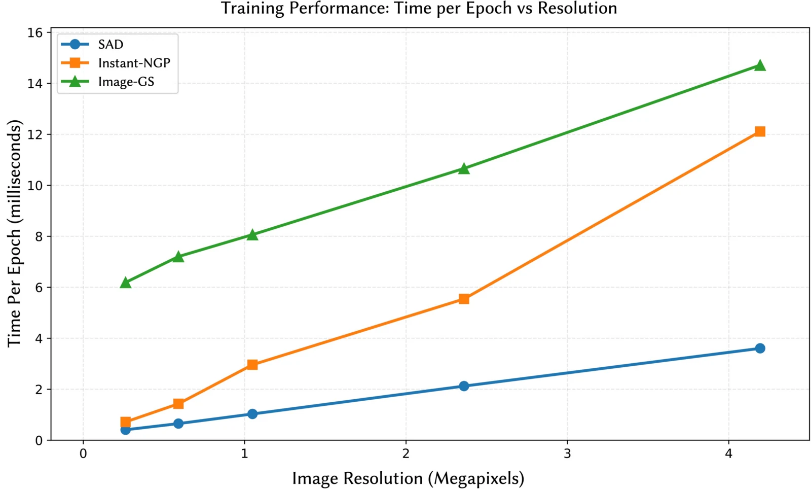
One epoch = one full pass over the pixels. SAD is fastest at every resolution: 1.75–3.36× over Instant-NGP and 4.08–15.10× over Image-GS; end to end, 4–19×.
How we keep cost per pixel constant
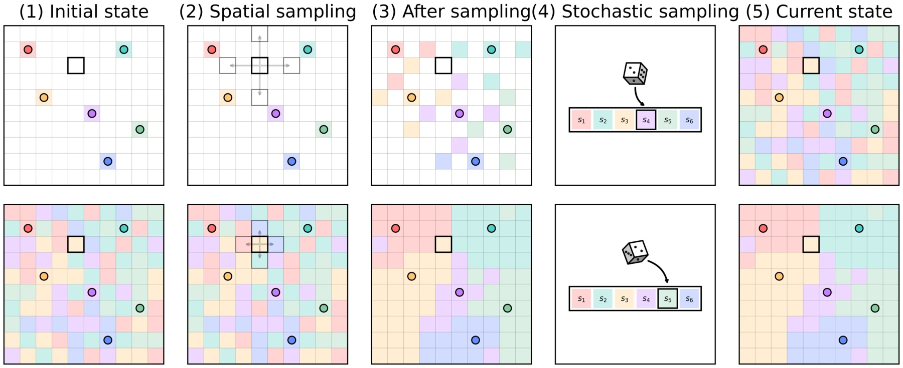
Evaluating all N sites per pixel is the thing that makes fitting slow. Instead we keep a per-pixel top-8 list under the shading score and refresh it: reuse the previous list, merge in candidates from the pixel and its four neighbours, and add a few global probes so a newly competitive distant site is not missed. The first passes follow a jump-flooding schedule; later refreshes are single-pass.
Every pass costs O(P·K), so encoding time does not grow with the site count the way a full nearest-neighbour search would, and the kernels stay regular.
Close-ups
DIV2K at 2.0 BPP. Drag the divider: the places that separate the methods are thin structures and hard-contrast edges, where a soft blend has to be sharpened rather than averaged. Error maps sit in the bottom-right corner of each panel.
left side
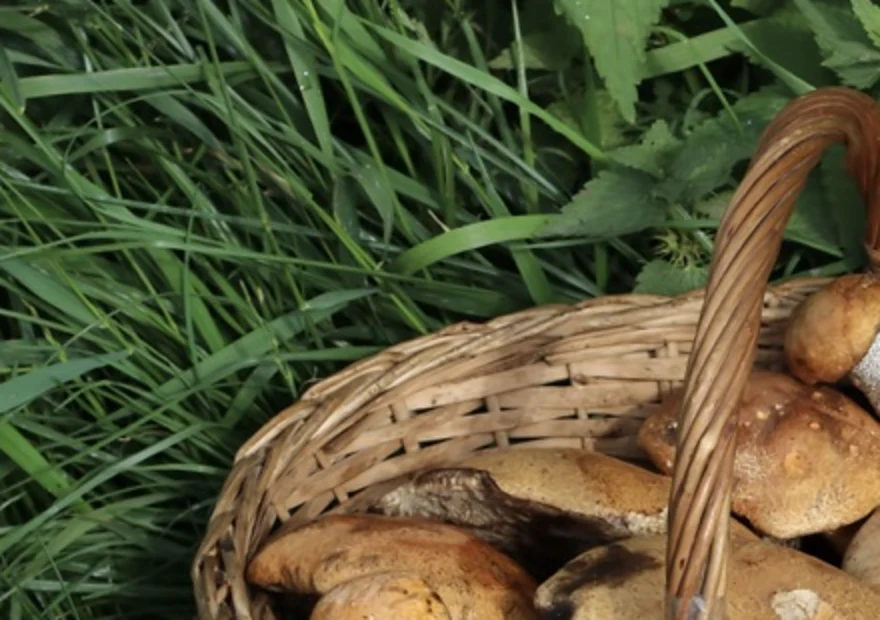
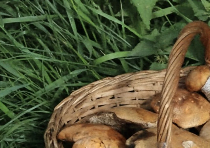
A 440×310 native crop of one DIV2K image at 2.0 BPP, shared by both panels; the divider reveals the same pixels under each method.
The same effect on site budget

What helps
Each learnable parameter in the score contributes something the others cannot. Turn them on one at a time: the cells change shape before the numbers change, and the last two settings are the ones that make the partition look like the image.

Diagram above, reconstruction below.
Average PSNR · five 2048² images at 0.5 BPP
35.35dB
+7.15 dB over the best fixed temperature.
- log τ learnable — +2.30 dB on its own. Sites covering a hard edge sharpen; sites covering a gradient stay soft.
- r learnable — +1.26 dB. Reach becomes a separate control from sharpness, so important cells can expand without getting blurrier.
- G learnable — +4.27 dB, the largest single gain. Cells elongate along image gradients, which is what a fixed isotropic ball cannot do.
The same mechanism at 1D: on a signal with a step, 64 sites reach 57.2 dB where a matched Gaussian-splat budget rounds the step off (47.3 dB) and a SIREN of comparable size rings around it (43.1 dB). The temperature sharpens exactly the discontinuity, and nothing else.
Beyond images
Because ownership is explicit, SAD can hold spatial constraints directly. Here it solves the 2D Poisson equation on an irregular domain: 20k interior sites plus 3k sites placed on the boundary contour, which are simply frozen after initialisation to enforce u = 0 exactly, with no penalty term and no level-set construction.

Gradient descent on the PDE residual reaches MSE < 10−6 in 1000–2000 steps.
The site-ID map is the interesting part: sites pile up along the boundary and around high curvature without being told where the boundary is, the same behaviour that puts them on edges in an image.
The representation is not tied to 2D images either; the 1D result above uses the same partition of unity over 64 sites with four parameters each.
Citation
@article{iinbor2026sad,
  title   = {Soft Anisotropic Diagrams for Differentiable Image Representation},
  author  = {Iinbor, Laki and Dou, Zhiyang and Matusik, Wojciech},
  journal = {ACM Transactions on Graphics},
  year    = {2026},
  note    = {SIGGRAPH 2026}
}